Axial Stretching

This case tests the axial stretching of a rod. The expected behavior is supposed to be like a spring-gravity motion, but with a rod. A rod is fixed at one end and a force is applied at the other end. The rod stretches and the displacement of the tip is compared with the analytical solution.

# isort:skip_file

import numpy as np
from matplotlib import pyplot as plt

import elastica as ea

Simulation Setup

We define a simulator class that inherits from the necessary mixins. This makes constraints, forces, and damping evailable to the system.

class StretchingBeamSimulator(
    ea.BaseSystemCollection, ea.Constraints, ea.Forcing, ea.Damping, ea.CallBacks
):
    pass


stretch_sim = StretchingBeamSimulator()
final_time = 200.0

Rod Setup

Next, we set up the test parameters for the simulating rods. This includes the number of elements, the start position, direction, normal, length, radius, density, and Young’s modulus of the rod. For this case, we have fixed boundary condition at one end, and we apply external force at the other end.

# setting up test params
n_elem = 19
start = np.zeros((3,))
direction = np.array([1.0, 0.0, 0.0])
normal = np.array([0.0, 1.0, 0.0])
base_length = 1.0
base_radius = 0.025
base_area = np.pi * base_radius**2
density = 1000
youngs_modulus = 1e4
# For shear modulus of 1e4, nu is 99!
poisson_ratio = 0.5
shear_modulus = youngs_modulus / (poisson_ratio + 1.0)

stretchable_rod = ea.CosseratRod.straight_rod(
    n_elem,
    start,
    direction,
    normal,
    base_length,
    base_radius,
    density,
    youngs_modulus=youngs_modulus,
    shear_modulus=shear_modulus,
)

stretch_sim.append(stretchable_rod)

stretch_sim.constrain(stretchable_rod).using(
    ea.OneEndFixedBC, constrained_position_idx=(0,), constrained_director_idx=(0,)
)

end_force_x = 1.0
end_force = np.array([end_force_x, 0.0, 0.0])
stretch_sim.add_forcing_to(stretchable_rod).using(
    ea.EndpointForces, 0.0 * end_force, end_force, ramp_up_time=1e-2
)

Damping is added to the system to help it reach a steady state. We use an AnalyticalLinearDamper to add damping to the rod.

# add damping
dl = base_length / n_elem
dt = 0.1 * dl
damping_constant = 0.1
stretch_sim.dampen(stretchable_rod).using(
    ea.AnalyticalLinearDamper,
    damping_constant=damping_constant,
    time_step=dt,
)

Callbacks

A callback object is passed to the simulator to record states of the rod during the simulation. This is useful for post-processing the results.

# Add call backs
class AxialStretchingCallBack(ea.CallBackBaseClass):
    """
    Tracks the velocity norms of the rod
    """

    def __init__(self, step_skip: int, callback_params: dict) -> None:
        super().__init__()
        self.every = step_skip
        self.callback_params = callback_params

    def make_callback(
        self, system: ea.typing.RodType, time: np.float64, current_step: int
    ) -> None:

        if current_step % self.every == 0:

            self.callback_params["time"].append(time)
            # Collect only x
            self.callback_params["position"].append(
                system.position_collection[0, -1].copy()
            )
            self.callback_params["velocity_norms"].append(
                np.linalg.norm(system.velocity_collection.copy())
            )
            return


recorded_history: dict[str, list] = ea.defaultdict(list)
stretch_sim.collect_diagnostics(stretchable_rod).using(
    AxialStretchingCallBack, step_skip=200, callback_params=recorded_history
)

Finalize and Run

We finalize the simulator and create the time-stepper. The PositionVerlet time-stepper is used to integrate the system.

stretch_sim.finalize()
timestepper: ea.typing.StepperProtocol = ea.PositionVerlet()
# timestepper = PEFRL()

total_steps = int(final_time / dt)
print("Total steps", total_steps)
dt = final_time / total_steps
time = 0.0
for i in range(total_steps):
    time = timestepper.step(stretch_sim, time, dt)

Total steps 38000

Post-Processing

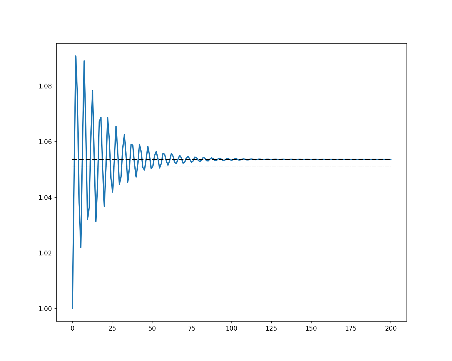
Finally, we plot the results and compare them with the analytical solution. The analytical solution is calculated using the first-order theory with both the base length and the modified length.

# First-order theory with base-length
expected_tip_disp = end_force_x * base_length / base_area / youngs_modulus
# First-order theory with modified-length, gives better estimates
expected_tip_disp_improved = (
    end_force_x * base_length / (base_area * youngs_modulus - end_force_x)
)

fig = plt.figure(figsize=(10, 8), frameon=True, dpi=150)
ax = fig.add_subplot(111)
ax.plot(recorded_history["time"], recorded_history["position"], lw=2.0)
ax.hlines(base_length + expected_tip_disp, 0.0, final_time, "k", "dashdot", lw=1.0)
ax.hlines(
    base_length + expected_tip_disp_improved, 0.0, final_time, "k", "dashed", lw=2.0
)
plt.show()