Butterfly

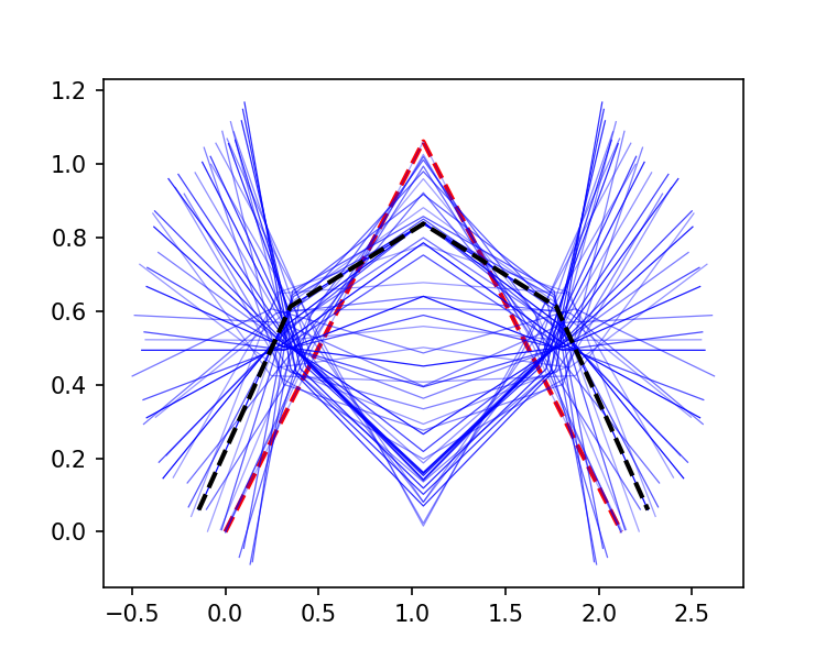
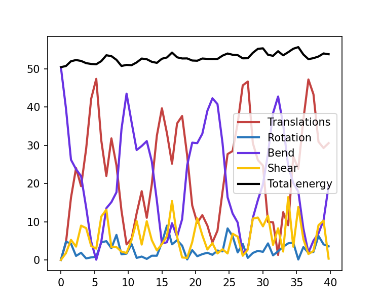
This case simulates the motion of a rod that is initially shaped like a butterfly. The rod is released from rest and allowed to deform freely. The goal of the simulation is for sanity check: how does the timestepper reliably preserve total energy of the system, when the system is simple Hamiltonian. The simulation tracks the position and energy of the rod over time.

This example case also demonstrate how to setup rod with customized positions and directors.

import numpy as np
from matplotlib import pyplot as plt
from matplotlib.colors import to_rgb


import elastica as ea
from elastica.utils import MaxDimension

Simulation Setup

We define a simulator class that inherits from the necessary mixins.

class ButterflySimulator(ea.BaseSystemCollection, ea.CallBacks):
    pass


butterfly_sim = ButterflySimulator()
final_time = 40.0

Rod Setup

Next, we set up the test parameters for the simulation.

# setting up test params
# FIXME : Doesn't work with elements > 10 (the inverse rotate kernel fails)
n_elem = 4  # Change based on requirements, but be careful
n_elem += n_elem % 2
half_n_elem = n_elem // 2

origin = np.zeros((3, 1))
angle_of_inclination = np.deg2rad(45.0)

# in-plane
horizontal_direction = np.array([0.0, 0.0, 1.0]).reshape(-1, 1)
vertical_direction = np.array([1.0, 0.0, 0.0]).reshape(-1, 1)

# out-of-plane
normal = np.array([0.0, 1.0, 0.0])

total_length = 3.0
base_radius = 0.25
base_area = np.pi * base_radius**2
density = 5000
youngs_modulus = 1e4
poisson_ratio = 0.5
shear_modulus = youngs_modulus / (poisson_ratio + 1.0)

We then define the initial positions of the nodes of the rod to create the butterfly shape.

positions = np.empty((MaxDimension.value(), n_elem + 1))
dl = total_length / n_elem

# First half of positions stem from slope angle_of_inclination
first_half = np.arange(half_n_elem + 1.0).reshape(1, -1)
positions[..., : half_n_elem + 1] = origin + dl * first_half * (
    np.cos(angle_of_inclination) * horizontal_direction
    + np.sin(angle_of_inclination) * vertical_direction
)
positions[..., half_n_elem:] = positions[
    ..., half_n_elem : half_n_elem + 1
] + dl * first_half * (
    np.cos(angle_of_inclination) * horizontal_direction
    - np.sin(angle_of_inclination) * vertical_direction
)

Now we can create the CosseratRod object with the specified positions.

butterfly_rod = ea.CosseratRod.straight_rod(
    n_elem,
    start=origin.reshape(3),
    direction=np.array([0.0, 0.0, 1.0]),
    normal=normal,
    base_length=total_length,
    base_radius=base_radius,
    density=density,
    youngs_modulus=youngs_modulus,
    shear_modulus=shear_modulus,
    position=positions,
)

butterfly_sim.append(butterfly_rod)

Callback Setup

A callback object is defined to record the position and energy of the rod during the simulation.

# Add call backs
class VelocityCallBack(ea.CallBackBaseClass):
    """
    Call back function for continuum snake
    """

    def __init__(self, step_skip: int, callback_params: dict) -> None:
        ea.CallBackBaseClass.__init__(self)
        self.every = step_skip
        self.callback_params = callback_params

    def make_callback(
        self, system: ea.typing.RodType, time: np.float64, current_step: int
    ) -> None:

        if current_step % self.every == 0:

            self.callback_params["time"].append(time)
            # Collect x
            self.callback_params["position"].append(system.position_collection.copy())
            # Collect energies as well
            self.callback_params["te"].append(system.compute_translational_energy())
            self.callback_params["re"].append(system.compute_rotational_energy())
            self.callback_params["se"].append(system.compute_shear_energy())
            self.callback_params["be"].append(system.compute_bending_energy())
            return


# database
recorded_history: dict[str, list] = ea.defaultdict(list)

# initially record history
recorded_history["time"].append(0.0)
recorded_history["position"].append(butterfly_rod.position_collection.copy())
recorded_history["te"].append(butterfly_rod.compute_translational_energy())
recorded_history["re"].append(butterfly_rod.compute_rotational_energy())
recorded_history["se"].append(butterfly_rod.compute_shear_energy())
recorded_history["be"].append(butterfly_rod.compute_bending_energy())

butterfly_sim.collect_diagnostics(butterfly_rod).using(
    VelocityCallBack, step_skip=100, callback_params=recorded_history
)

Finalize and Run

We finalize the simulator and create the time-stepper.

butterfly_sim.finalize()
timestepper: ea.typing.StepperProtocol
timestepper = ea.PositionVerlet()
# timestepper = PEFRL()

dt = 0.01 * dl
total_steps = int(final_time / dt)
print("Total steps", total_steps)
dt = final_time / total_steps
time = 0.0
for i in range(total_steps):
    time = timestepper.step(butterfly_sim, time, dt)

Total steps 5333

Post-Processing

The position of the rod is plotted at different time steps, and the energies are plotted as a function of time.

# Plot the histories
fig = plt.figure(figsize=(5, 4), frameon=True, dpi=150)
ax = fig.add_subplot(111)
positions_history = recorded_history["position"]
# record first position
first_position = positions_history.pop(0)
ax.plot(first_position[2, ...], first_position[0, ...], "r--", lw=2.0)
n_positions = len(positions_history)
for i, pos in enumerate(positions_history):
    alpha = np.exp(i / n_positions - 1)
    ax.plot(pos[2, ...], pos[0, ...], "b", lw=0.6, alpha=alpha)
# final position is also separate
last_position = positions_history.pop()
ax.plot(last_position[2, ...], last_position[0, ...], "k--", lw=2.0)
# don't block
fig.show()

# Plot the energies
energy_fig = plt.figure(figsize=(5, 4), frameon=True, dpi=150)
energy_ax = energy_fig.add_subplot(111)
times = np.asarray(recorded_history["time"])
te = np.asarray(recorded_history["te"])
re = np.asarray(recorded_history["re"])
be = np.asarray(recorded_history["be"])
se = np.asarray(recorded_history["se"])

energy_ax.plot(times, te, c=to_rgb("xkcd:reddish"), lw=2.0, label="Translations")
energy_ax.plot(times, re, c=to_rgb("xkcd:bluish"), lw=2.0, label="Rotation")
energy_ax.plot(times, be, c=to_rgb("xkcd:burple"), lw=2.0, label="Bend")
energy_ax.plot(times, se, c=to_rgb("xkcd:goldenrod"), lw=2.0, label="Shear")
energy_ax.plot(times, te + re + be + se, c="k", lw=2.0, label="Total energy")
energy_ax.legend()
# don't block
energy_fig.show()

plt.show()